Reading Notes: Probabilistic Model-Agnostic Meta-Learning

This post is a reading note for the paper "Probabilistic Model-Agnostic Meta-Learning" by Finn et al. It is a successive work to the famous MAML paper, and can be viewed as the Bayesian version of the MAML model.

Introduction

When dealing with different tasks of the same family, for example, the image classification family, the neural language processing family, etc.. It is usually preferred to be able to acquire solutions to complex tasks from only a few samples given the past knowledge of other tasks as a prior (few shot learning). The idea of learning-to-learn, i.e., meta-learning, is such a framework.

What is meta-learning?

The model-agnostic meta-learning (MAML) [1] is a few shot meta-learning algorithm that uses gradient descent to adapt the model at meta-test time to a new few-shot task, and trains the model parameters at meta-training time to enable rapid adaptation.

The idea is that we assume there are some tasks that are drawn from some distribution $p(\mathcal{T})$. For each task $\mathcal{T}_i\sim p(\mathcal{T})$, we sample the data into two sets, $\mathcal{D}^{tr}$ and $\mathcal{D}^{test}$, where $\mathcal{D}^{tr}$ is used for training the model, and $\mathcal{D}^{test}$ is for measuring whether or not the training was effective.

The MAML algorithm trains for few-shot generalization by optimizing for a set of initial parameters $\theta$ such that one or a few steps of gradient descent on a $\mathcal{D}^{tr}$ achieves good performance on $\mathcal{D}^{test}$. The objective function to optimize MAML is

$\min _{\theta} \sum_{\mathcal{T}_{i} \sim p(\mathcal{T})} \mathcal{L}\left(\theta-\alpha \nabla_{\theta} \mathcal{L}\left(\theta, \mathcal{D}_{\mathcal{T}_{i}}^{\mathrm{tr}}\right), \mathcal{D}_{\mathcal{T}_{i}}^{\mathrm{test}}\right)=\min _{\theta} \sum_{\mathcal{T}_{i} \sim p(\mathcal{T})} \mathcal{L}\left(\phi_{i}, \mathcal{D}_{\mathcal{T}_{i}}^{\mathrm{test}}\right)$,

where $\phi_i$ is used to denote the parameters updated by gradient descent and where the loss corresponds to negative log likelihood of the data.

Note that this objective function is different from the traditional learning objective functions in terms of

1. There are 2 gradients to calculate for each updates, one from $\mathcal{D}^{tr}$, and the other from $\mathcal{D}^{test}$;
2. The loss is calculated based on current parameter set $\theta$ plus $-\alpha \nabla_{\theta} \mathcal{L}\left(\theta, \mathcal{D}_{\mathcal{T}_{i}}^{\mathrm{tr}}\right)$, it essentially means the parameter of a model that is 1-step trained with $\mathcal{D}^\mathrm{tr}$.

Bayesian Meta-learning

When the end goal of few-shot meta-learning is to learn solutions to new tasks from small amounts of data, a critical issue that must be dealt with is task ambiguity: even with the best possible prior, there might be still not enough information from these few data points to resolve the new task with high certainty. Hence it is desirable to be able to sample multiple solutions with some uncertainty. Such a method could be used to evaluate uncertainty (by measuring agreement between the samples), perform active learning, or elicit direct human supervision about which sample is preferable.

The hierarchical Bayesian model

The hierarchical Bayesian is designed that includes random variables for the prior distribution over function parameters, $\theta$, the distribution over parameters for a particular task, $\phi_i$ , and the task training and test datapoints.

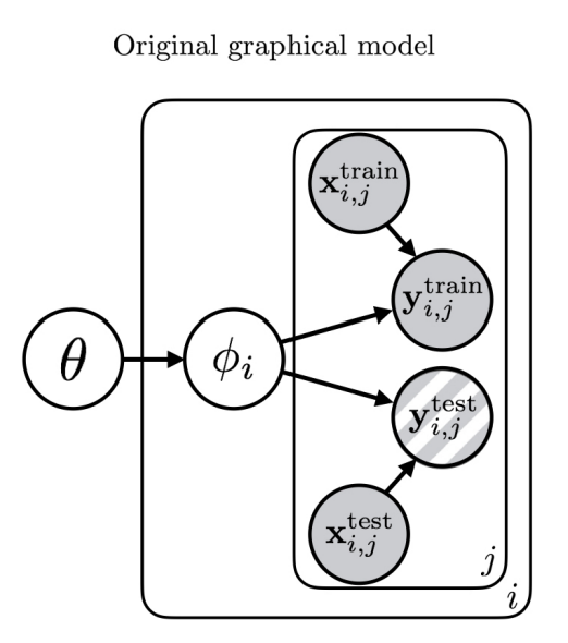
Fig 1: Hierarchical model with meta prior $\theta$ and task parameter $\phi_i$.

Gradient-Based Meta-Learning with Variational Inference

One straightforward way is to combine meta-learning with variational inference. We approximate the distribution over the hidden variables $\theta$ and $\phi_i$ for each task with some distribution $q_i(\theta, \phi_i)$. And further rewrite it as $q_i(\theta,\phi_i)=q_i(\theta)q_i(\phi_i)$. The variational lower bound on the log-likelihood can be written as

$\begin{aligned} \log p\left(\mathbf{y}_{i}^{\text {test }} | \mathbf{x}_{i}^{\text {test }}, \mathbf{x}_{i}^{\text {tr }}, \mathbf{y}_{i}^{\text {tr }}\right) \geq & \underset{\theta, \phi_{i} \sim q_{\psi}}{\mathbb{E}}\left[\log p\left(\mathbf{y}_{i}^{\text {tr }} | \mathbf{x}_{i}^{\text {tr }}, \phi_{i}\right)+\log p\left(\mathbf{y}_{i}^{\text {test }} | \mathbf{x}_{i}^{\text {test }}, \phi_{i}\right)+\log p\left(\phi_{i} | \theta\right)+\log p(\theta)\right]+\\ & \mathcal{H}\left(q_{\psi}\left(\phi_{i} | \theta, \mathbf{x}_{i}^{\text {tr }}, \mathbf{y}_{i}^{\text {tr }}, \mathbf{x}_{i}^{\text {test }}, \mathbf{y}_{i}^{\text {test }}\right)\right)+\mathcal{H}\left(q_{\psi}\left(\theta | \mathbf{x}_{i}^{\text {tr }}, \mathbf{y}_{i}^{\text {tr }}, \mathbf{x}_{i}^{\text {test }}, \mathbf{y}_{i}^{\text {test }}\right)\right) \end{aligned}$

where $q_{\psi}\left(\phi_{i} | \theta, \mathbf{x}_{i}^{\text {tr }}, \mathbf{y}_{i}^{\text {tr }}, \mathbf{x}_{i}^{\text {test }}, \mathbf{y}_{i}^{\text {test }}\right)$ and $q_{\psi}\left(\theta | \mathbf{x}_{i}^{\text {tr }}, \mathbf{y}_{i}^{\text {tr }}, \mathbf{x}_{i}^{\text {test }}, \mathbf{y}_{i}^{\text {test }}\right)$ are neural inference network approximations to $q_i(\phi_i|\theta)$ and $q_i(\theta)$.

These inference networks can be constructed by

$q_{\psi}\left(\theta | \mathbf{x}_{i}^{\mathrm{tr}}, \mathbf{y}_{i}^{\mathrm{tr}}, \mathbf{x}_{i}^{\mathrm{test}}, \mathbf{y}_{i}^{\mathrm{test}}\right)=\mathcal{N}\left(\boldsymbol{\mu}_{\theta}+\boldsymbol{\gamma}_{q} \nabla_{\mu_{\theta}} \log p\left(\mathbf{y}_{i}^{\mathrm{tr}} | \mathbf{x}_{i}^{\mathrm{tr}}, \boldsymbol{\mu}_{\theta}\right)+\boldsymbol{\gamma}_{q} \nabla_{\mu_{\theta}} \log p\left(\mathbf{y}_{i}^{\mathrm{test}} | \mathbf{x}_{i}^{\mathrm{test}}, \boldsymbol{\mu}_{\theta}\right) ; \mathbf{v}_{q}\right)$

However, in this approach, at the meta-test time, we must obtain the posterior $p(\phi_i |x^{tr}_i, y^{tr}_i , x^{test}_i )$, without access to $y^{test}_i$ . We can train a separate set of inference networks to perform this operation, potentially also using gradient descent within the inference network. However, these networks do not receive any gradient information during meta-training, and may not work well in practice.

Probabilistic Model-Agnostic Meta-Learning Approach with Hybrid Inference

MAML can be interpreted as approximate inference for the posterior

$p\left(\mathbf{y}_{i}^{\mathrm{test}} | \mathbf{x}_{i}^{\mathrm{tr}}, \mathbf{y}_{i}^{\mathrm{tr}}, \mathbf{x}_{i}^{\mathrm{test}}\right)=\int p\left(\mathbf{y}_{i}^{\mathrm{test}} \mathbf{x}_{i}^{\mathrm{test}}, \phi_{i}\right) p\left(\phi_{i} | \mathbf{x}_{i}^{\mathrm{tr}}, \mathbf{y}_{i}^{\mathrm{tr}}, \theta\right) d \phi_{i} \approx p\left(\mathbf{y}_{i}^{\mathrm{test}} | \mathbf{x}_{i}^{\mathrm{test}}, \phi_{i}^{\star}\right)$

where $\phi^\star_i$ is the maximum a posteriori (MAP) value. This can be viewed as the dependency network shown in Fig 2.

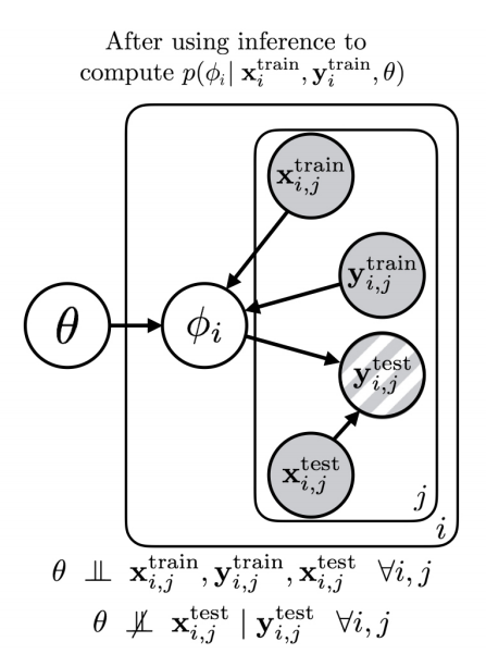
Fig 2: the dependency network after inference.

Thus, we can now write down a variational lower bound for the logarithm of the approximate likelihood, which is given by

$\log p\left(\mathbf{y}_{i}^{\text {test }} | \mathbf{x}_{i}^{\text {test }}, \mathbf{x}_{i}^{\text {tr }}, \mathbf{y}_{i}^{\text {tr }}\right) \geq E_{\theta \sim q_{\psi}}\left[\log p\left(\mathbf{y}_{i}^{\text {test }} | \mathbf{x}_{i}^{\text {test }}, \phi_{i}^{\star}\right)+\log p(\theta)\right]+\mathcal{H}\left(q_{\psi}\left(\theta | \mathbf{x}_{i}^{\text {test }}, \mathbf{y}_{i}^{\text {test }}\right)\right)$

Analogously to the previous section, the inference network is given by

$q_{\psi}\left(\theta | \mathbf{x}_{i}^{\text {test }}, \mathbf{y}_{i}^{\text {test }}\right)=\mathcal{N}\left(\boldsymbol{\mu}_{\theta}+\gamma_{q} \nabla \log p\left(\mathbf{y}_{i}^{\text {test }} | \mathbf{x}_{i}^{\text {test }}, \boldsymbol{\mu}_{\theta}\right) ; \mathbf{v}_{q}\right)$

At meta-test time, the inference procedure is much simpler. The test labels are not available, so we simply sample $\theta \sim p(\theta)$ and perform MAP inference on $\phi_i$ using the training set, which corresponds to gradient steps on $\log p(y_i^{tr}|x_i^{tr}, \theta_{current})$, where $\theta_{current}$ starts at the sampled $\theta$. The procedure is described in Algorithm 1.

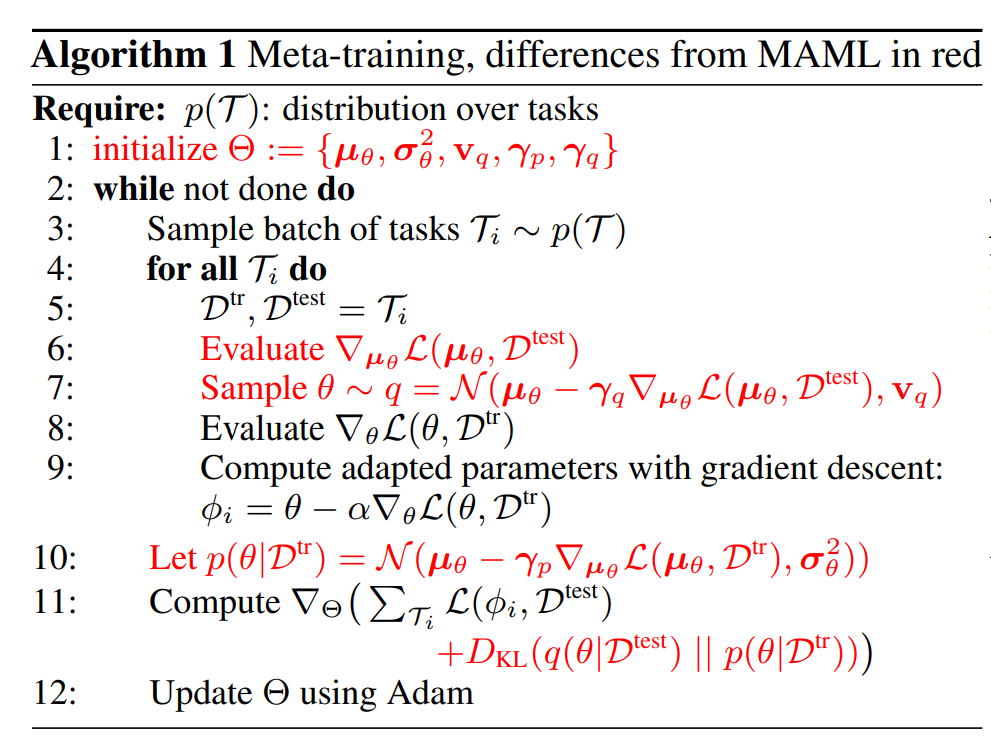
Algorithm 1: Probabilistic MAML

Adding additional dependencies

To remedy the crude approximation to $p(\phi_i|x)i^{tr}, y_i^{tr}, \theta)$, the authors propose additional dependencies in the dependency graph, as shown in Fig 3.

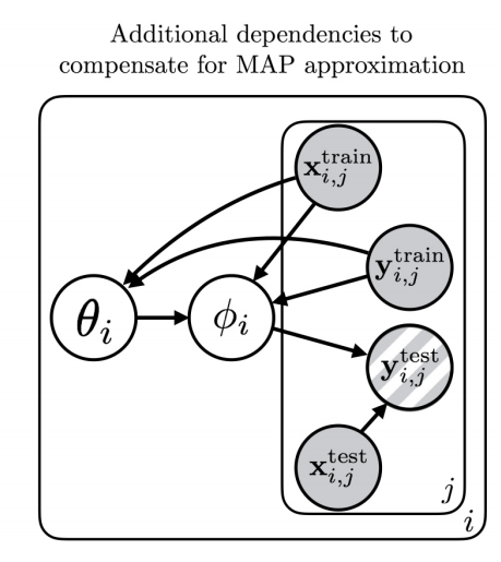
Fig 3: additional dependencies to compensate for MAP approximation.

Here $\theta_i$ is proposed to be dependent on $x_i^{tr}$ and $y_i^{tr}$, the inference network $q_\psi$ can be constructed as

$p\left(\theta_{i} | \mathbf{x}_{i}^{\mathrm{tr}}, \mathbf{y}_{i}^{\mathrm{tr}}\right)=\mathcal{N}\left(\boldsymbol{\mu}_{\theta}+\boldsymbol{\gamma}_{p} \nabla \log p\left(\mathbf{y}_{i}^{\mathrm{tr}} | \mathbf{x}_{i}^{\mathrm{tr}}, \boldsymbol{\mu}_{\theta}\right) ; \boldsymbol{\sigma}_{\theta}^{2}\right)$

According to the experiments done by the authors, this more expressive distribution often leads to better performance. This meta-testing part is shown in Algorithm 2.

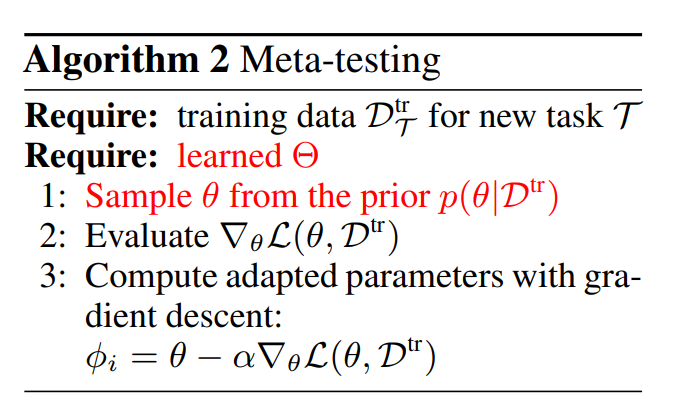
Algorithm 2: meta-testing part.

[1] Finn, Chelsea, Pieter Abbeel, and Sergey Levine. "Model-agnostic meta-learning for fast adaptation of deep networks." Proceedings of the 34th International Conference on Machine Learning-Volume 70. JMLR. org, 2017.