Reading Notes: Copulas as High-Dimensional Generative Models: Vine Copula Autoencoders

Copulas as High-Dimensional Generative Models: Vine Copula Autoencoders

This post is a work through for this paper by Natasa et al: Copulas as High-Dimensional Generative Models: Vine Copula Autoencoders, one can find the paper here.

Introduction

The authors introduced vine copula autoencoder (VCAE) as a flexible generative model for high-dimensional distributions. The model is simply built in a three-step procedure:

1. Train an autoencoder to compress the data into a lower dimensional representations;
2. Estimate the encoded representation's distribution with vine copulas;
3. Combine the distribution and the decoder to generate new data points.

The authors claimed that this generative model has 3 advantages compared to Generative Adversarial Nets (GANs) and Variational Autoencoders (VAEs):

1. It offers modeling flexibility by avoiding most distributional assumptions in contrast to VAEs;
2. Training and sampling procedures for high-dimensional data are straightforward;
3. It can be used as a plug-in allowing to turn any AE into generative model, simultaneously allowing it to serve other purposes (e.g., denoising, clustering).

Vine copula autoencoders

The basic procedure of training vine copula autoencoders (VCAE) is described in Fig 1. The first building block of VCAE is a regular autoencoder, with a compressed latent representation $z$. One major difference between VCAE and VAE is that VAEs assume a simple prior (like Gaussian) to $z$, however, VCAEs doesn't make such assumptions, they deal with the distribution entirely with vine copula training.

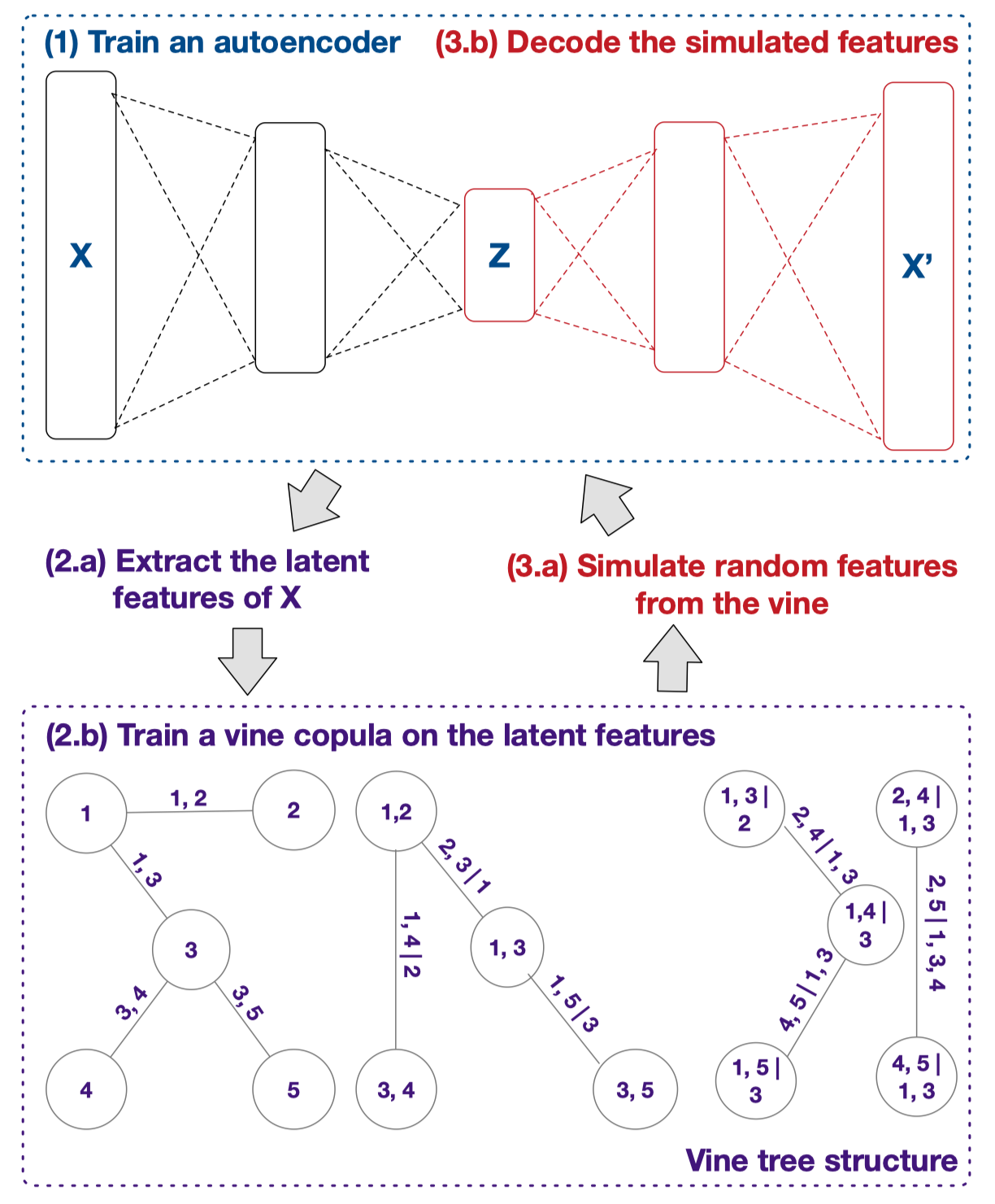
Fig 1: Conceptual illustration of a VCAE.

If we use $X' \approx g(f(X))$ to represent the autoencoder, then the job of vine copula is to learn the distribution of $z$ such that it can generate samples using $X' = g(z)$.

Vine copulas

The major contribution lies in the application of vine copulas.

Copulas and its basic property

The Sklar's theorem tells us that copulas allow us to decompose a joint density into a product between the marginal densities $f_i$ and the dependence structure represented by the copula density $c$. i.e., assuming that all densities exist, we can write $f\left(x_{1}, \ldots, x_{d}\right)=c\left\{u_{1}, \ldots, u_{d}\right\} \times \prod_{k=1}^{d} f_{k}\left(x_{k}\right)$, where $u_i = F_i(x_i)$ and $f, c, f_1,...,f_d$ are the densities corresponding to $F, C, F_1,...,F_d$ respectively.

This implies that the generating procedure can be done in two steps:

1. Estimating the marginal distributions;
2. Using the estimated distributions to construct pseudo-observations via the probability integral transform before estimating the copula density.

Vine copulas construction

The pair-copula constructions (PCCs), also called vine copulas, is used in this paper as pair wise copula construction is much more feasible compared to joint modeling all variables.

PCCs model the joint distribution of a random vector by decomposing the problem into modeling pairs of conditional random variables, making the construction of complex dependencies both flexible and yet tractable.

Lets consider an example with 3 random variables $(X_1, X_2, X_3)$, the joint density $f$ of $X$ can be decomposed as

$$f = f_1f_2f_3c_{1,2}c_{2,3}c_{1,3|2}$$

Where $f_i$s represents the marginal distributions of $X_i$, and $c_{i,j}$ represents the pair copula between $X_i$ and $X_2$, which also represents the dependencies. Note that $c_{1,3|2}$ represents conditional copula/dependency.

For the details of how vine copulas are estimated, or why they would work, one can read the workshop slides by Nicole et al. in NIPS workshop 2011.

The training and generating procedure of vine copula

Fig 2 illustrate the estimation and sampling procedure for a (conditional) pair copula.

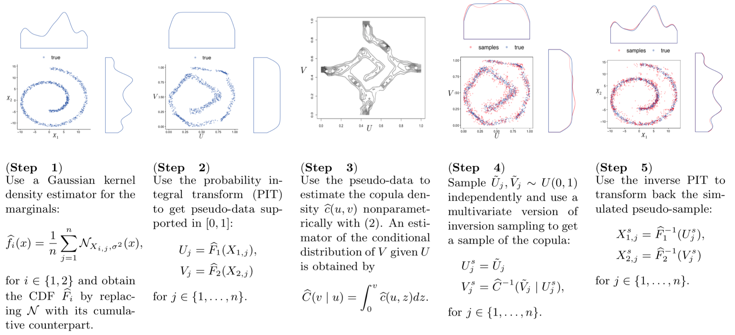
Fig 2: Estimation and sampling algorithm for a pair copula

Note that plenty of the algorithms for vine copula estimation and generation are implemented in C++ package vinecopulib.

 

Conclusion

The authors proposed a new way for deep generative modeling using vine copulas with a very clever combination of traditional vine copula estimation and a regular auto encoder modeling. This inspires us to apply more old-school techniques on the latent low-dimensional features learned by deep networks like autoencoders.