Evaluation methods for recommender systems

There are plenty of recommender systems available, the question is, for a specific recommendation problem, which recommender system model to use? The prediction accuracy (ratio of correct predicted items) is a straightforward approach, however, this is in most cases doesn't give a good indication on how 'good' the model is? Because usually, the ratings are somehow ordinal, which means the ratings are ordered instead of categorical, a prediction of 4 star is better than prediction of 5 star for a ground truth of 3 star, while when evaluate with accuracy, 4-star prediction and 5-star are treated equal -- incorrect prediction.

There are plenty of better evaluation methods available,  in this post, I will introduce some of them. But first of all, lets review some basic concepts in model evaluation.

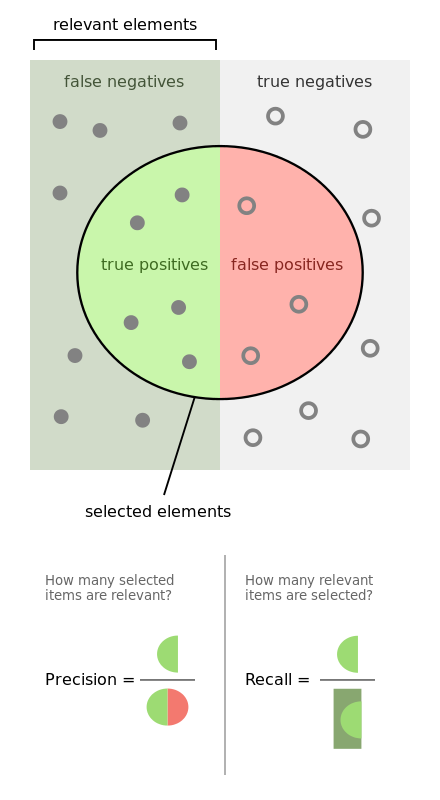
To simplify our settings, lets say that we have a binary classification model, it made predictions on a test dataset, the prediction result is shown in Figure 1. Then the precision, recall, sensitivity and specificity are defined as follows respectively.

• Precision:  The probability that a selected item is positive. \[\text{precision} = \frac{TP}{TP + FP}\]

• Recall: The probability that a positive is selected.   \[\text{recall} = \frac{TP}{TP+FN}\]

Figure 1a. Precision and Recall
Credit: wikipedia

• Sensitivity: Also called true positive rate (TPR), is equivalent to Recall, it measures how many positive items are selected. \[\text{Sensitivity} = \frac{TP}{TP+FN}\]
• Specificity: Also called true negative rate (TNR),  how many negative selected items are truly negative. \[\text{Specificity} = \frac{TN}{TN + FP}\]

Figure 1b. Sensitivity and Specificity
Credit: wikipedia

Root-Mean-Square Error (RMSE)

Also called root-mean-square deviation (RMSD). The RMSE is defined by the root of mean-square-error, assume $\theta$ is the target value, and $\hat{\theta}}$ the estimated value, the RMSE is defined by:
\[\operatorname{RMSD}(\hat{\theta}) = \sqrt{\operatorname{MSE}(\hat{\theta})} = \sqrt{\operatorname{E}((\hat{\theta}-\theta)^2)}.\]
For an unbiased estimator, RMSE is equivalent to the standard deviation of estimator.

Precision-Recall Curve and ROC

The receiver operating characteristic curve (ROC curve) is a graphical plot that illustrates the diagnostic ability of a binary classifier system as its discrimination threshold is varied.  The ROC is created by plotting the true positive rate (TPR) versus the false positive rate (FPR). True positive rate is also called sensitivity, and false positive rate is also called fall-out, and is equivalent to (1 - specificity).

Figure 2. ROC curve of three predictors of peptide cleaving in the proteasome.

For a good classifier, it should has both reasonably high sensitivity and specificity. In terms of ROC curve, it means the curve should be as close to top left as possible. (Because FPR is equal to (1 - specificity), the points at top left corner indicates both high sensitivity and high specificity).

Area Under the Curve (AUC)

When using normalized units, the area under the curve (often referred to as simply the AUC) is equal to the probability that a classifier will rank a randomly chosen positive instance higher than a randomly chosen negative one. (credit: wikipedia)

Precision-Recall Curve

Precision at k considers top k results returned by the model. It is a term from Information Retrieval, we can understand it as the proportion of recommended items in the top-k set that are relevant.

Similarly recall at k is the proportion of relevant items found in the top-k recommendations.

The precision-recall curve (PR curve) as the name indicates, is a graphical plot that created by plotting the precision versus recall, at each k. This curve illustrates the trade-off between precision and recall.

Mean Average Precision

Let's first introduce average precision, suppose there is a precision-recall curve, and follows a function $p = p(r)$, where $p$ and $r$ represents precision and recall respectively.  Then the average precision is defined by

\[\operatorname{AveP} = \int_0^1 p(r)dr\]

It can also be viewed as the area under the precision-recall curve.

The mean average precision (MAP) is the mean of average precision over all users. For example, a recommender could recommend a list of items for a user, for this user, there is a precision-recall curve, hence average precision, MAP is the mean of all average precisions over all users. (In the contexts of Information Retrieval, MAP is the mean of average precisions over all queries)

\[\operatorname{MAP} = \frac{\sum_{u=1}^N \operatorname{AveP(u)}}{N} \!\]

Normalized Discounted Cumulative Gain (nDCG)

Before digging into NDCG, we must first introduce discounted cumulative gain (DCG) and cumulative gain (CG).

Cumulative Gain (CG) is the sum of graded relevances of all results in the returned list. Graded relevance is manually given by the user, the scale is not restricted, which makes the CG not comparable between different models, the simplest definition is binary $rel_i \in \{0,1\}$. The CG can be written as

\[{\mathrm {CG_{{p}}}}=\sum _{{i=1}}^{{p}}rel_{{i}}\]

Where $rel_{i}$ is the graded relevance of the result at position

The discounted cumulative gain (DCG) takes a step further, it considers the rank within the returned list, as the results ranked at the top of the list should be ideally more relevant than results near the tail. Hence DCG takes discounts on the graded relevances based on the rank of the results. The DCG is defined by

\[\text{DCG}_p = rel_1 + \sum_{i=2}^p \frac{rel_i}{\log_2{i}}\]

The normalized discounted cumulative gain (nDCG) is generally normalized using the ideal DCG, it is widely used in industry including major web search engines, and data science competition platforms such as Kaggle (credit: wikipedia). The IDCG is defined by

\[{\displaystyle \mathrm {IDCG_{p}} =\sum _{i=1}^{|REL|}{\frac {2^{rel_{i}}-1}{\log _{2}(i+1)}}}\]

and |REL| represents the list of relevant documents (ordered by their relevance) in the corpus up to position p. And hence the nDCG is

\[{\mathrm {nDCG_{{p}}}}={\frac {DCG_{{p}}}{IDCG_{{p}}}},\]